Architectures
August 2026 – Vladislav KruglikovNeural network architectures are built from components that transform representations and control how information flows through the model. This article collects short explanations of these components, starting with dropout.
Dropout
Dropout randomly sets part of an activation tensor to zero during training. It is a regularizer. The model cannot rely on every feature always being present, so it is pushed to learn less brittle representations.
During training, each value is kept with probability and dropped with probability . The kept values are divided by :
where is a random mask with values or .
The scaling keeps the expected value the same. For one activation :
That is why in evaluation dropout does nothing but in training samples a mask and rescales the kept activations.
In distributed training, replicated activations that must remain identical need the same dropout mask on every replica. Different shards of one activation instead use independent mask entries, so together they form one independent mask for the full tensor.
Dropout should usually come after the activation because some activations turn an input of zero into a nonzero output. For example, , so masking a value before sigmoid does not actually remove it. Masking after the activation always makes the dropped feature zero. With ReLU the two placements can be equivalent because .
Applying dropout after the final logits usually does not make sense. Logits are the direct inputs to the loss. If we randomly zero them, we are corrupting the model's answer right before the objective reads it.
- Analysis of Dropout
- Improving neural networks by preventing co-adaptation of feature detectors, the original Dropout paper.
Residual connection
A residual block is a group of layers with a shortcut connection that adds the original input to the layers' output. If the layers compute , the block returns .
During the backward pass, the gradient can flow through both paths. Let and let be the Jacobian of . Then
The first term is the gradient through , and the second is the gradient through the identity shortcut.
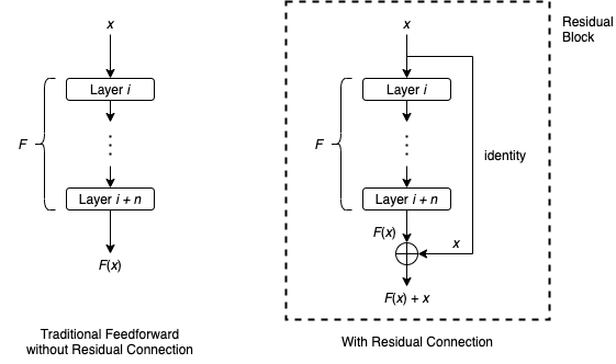
Suppose the desired output for input is the underlying mapping . Instead of asking the stacked layers to learn directly, a residual block lets them learn a residual function relative to the input. The original mapping is then obtained by adding the input back:
The idea is that optimizing the residual mapping can be easier than optimizing the original, unreferenced mapping. If the identity mapping is already a good solution, so that , the stacked layers only need to push toward zero. This can be easier than learning the identity function from scratch through multiple nonlinear layers. The Deep Residual Learning paper introduced this approach.
Attention
Attention produces each token's new representation as a weighted sum of the hidden states of other tokens. For token , it has the form:
Here is the value representation of token , and is the weight that token assigns to it. The weights are computed afresh for each input from query-key similarity scores and normalized with softmax. Training learns the query, key, and value projections that produce those scores, so the model learns how to assign useful weights rather than learning one fixed set of weights for every sequence.
Feed-forward network (FFN)
The feed-forward network is the Transformer block's per-token feature extractor. Attention mixes information across tokens, while the FFN transforms each token representation independently. A standard FFN expands the hidden size from to a larger intermediate size , applies a nonlinearity, then projects back to :
In a Transformer block, the FFN follows multi-head attention. Attention gathers information from other tokens, and its output projection combines the attention heads. The FFN then mixes those combined features within each token and creates new nonlinear features for the next block.
The intermediate dimension is usually larger than the model dimension, often . Reducing it below would create a bottleneck that compresses the representation before the model can form many useful features. The up projection gives the nonlinearity more feature directions to combine, and the down projection returns the result to the fixed hidden size required by the residual stream.
The choice of roughly is an empirical capacity–cost tradeoff. With input features, even considering pairwise relationships gives on the order of possible interactions. A network cannot explicitly represent every possible interaction, but a very narrow intermediate layer would leave it with too few nonlinear features to represent many useful combinations. Expanding the width gives the FFN room to develop more patterns before projecting them back, while keeping the parameter count and compute practical.
Multi-head attention (MHA)
MHA gives every attention head its own query, key, and value projections. The heads can learn different relationships, then their outputs are concatenated and mixed. This is the attention mechanism introduced in Attention Is All You Need.
Grouped-query attention (GQA)
GQA keeps many query heads but groups them so that several query heads share one key and value head. It reduces key/value cache memory and bandwidth while retaining more query-head diversity than MQA. See GQA: Training Generalized Multi-Query Transformer Models from Multi-Head Checkpoints.
Multi-query attention (MQA)
MQA gives every query head its own projection but shares a single key and value head across all queries. This greatly reduces key/value cache size and decoding bandwidth, at the cost of less independent key/value representations. It was introduced in Fast Transformer Decoding: One Write-Head is All You Need.
Multi-head latent attention (MLA)
MLA compresses each token's key and value information into a smaller latent vector, then reconstructs the head-specific representations when computing attention. The KV cache stores the latent vectors instead of every key and value head, reducing memory and decoding bandwidth while preserving more head diversity than MQA. It was introduced in DeepSeek-V2.
Sliding-window attention
Sliding-window attention (SWA) restricts each token to attending only to nearby tokens. In a causal decoder, query token attends to keys in the preceding window , where is the window size. The Longformer popularized a sliding-window attention design for long documents, combined with selected global attention links. Local attention predates Longformer, but Longformer made this sparse pattern a practical drop-in replacement for full attention.
In practice, SWA is often interleaved with full-attention layers. Using sliding windows everywhere would reduce the cost further, but a token could no longer directly retrieve information from distant parts of the prompt. Full-attention layers preserve these long-range retrieval paths while most layers keep the cheaper local pattern.
In forward, the attention kernel computes query-key scores and the weighted value sum only for the window edges. It does not materialize the full attention matrix. In backward, the same sparse edges receive gradients: each query, key, and value is differentiated only through the windowed attention pairs that existed in forward. Stacking layers expands the receptive field, so information can travel roughly tokens across local-attention layers.
For a sequence of length , full attention has attention-score work per layer in both training forward and backward. SWA reduces this to . During inference, prompt prefill falls from to . After the cache has reached the window size, each generated token has attention work and key–value reads instead of , and the per-layer KV cache can remain instead of growing as .
Linear attention
In practice, linear attention is often combined with full-attention layers. Its fixed-size state gives predictable memory and compute as the context grows, but compressing the past into that state can make it harder to retrieve an arbitrary distant token exactly. Full-attention layers restore direct long-range access while the linear layers keep most of the sequence processing cheaper.
Further reading:
Attention sinks
Keeping only the most recent window can make a streaming language model unstable once the context exceeds the cache size. Attention sinks keep a small number of initial token KVs permanently, together with the latest token KVs. Initial tokens often receive high attention even when they are not semantically important, acting as a place for excess attention probability to go. Every new query can attend to the sink tokens and its local window, giving decode work and bounded cache memory while preserving stable long-stream behavior.
PostNAS and Jet-Nemotron
Jet-Nemotron uses PostNAS to search for an efficient hybrid language-model architecture starting from a pretrained full-attention model. The search can choose which layers retain full attention, which use linear attention, and which new attention blocks to introduce, while also considering hardware-aware hyperparameters. This treats the placement of attention mechanisms as a search problem rather than a fixed architectural choice.
Encoder–decoder architecture
An encoder–decoder model runs an encoder over the input once, then generates output tokens with an autoregressive decoder that cross-attends to the encoder states. This split can improve inference speed for generation-heavy workloads. Suppose an encoder–decoder model has the same total parameter budget as a decoder-only model, but two-thirds of its parameters are in the encoder and one-third are in the decoder. The encoder work is paid once for the input, while the smaller decoder runs once for every generated token. The original T5 paper uses this encoder–decoder Transformer design for text-to-text tasks.
Generation is often memory-bandwidth-bound because each new token requires reading decoder weights and key–value cache data from HBM. A smaller decoder means less weight traffic on every decode step, so it can generate tokens faster. This is most useful when decoding dominates latency, such as long outputs with short or moderate inputs. The encoder prefill can be larger, but it is a one-time cost rather than work repeated for every generated token.
Weight tying
Language models usually have an input embedding matrix and a separate output projection, or language-model head. Both have one vector per vocabulary token. When the vocabulary is large relative to the rest of a small model, these two matrices can dominate parameter and memory use. Weight tying reuses the input embedding matrix for the output projection instead of learning a second vocabulary-sized matrix:
Here is the hidden state at position , is an output bias, and contains one logit for every token. The logit for token is the dot product of with the embedding of . Softmax therefore ranks tokens by their similarity to the hidden state, much like a similarity search in the token-embedding space. Tying also encourages tokens with similar embeddings to receive similar predictions.
In an autoregressive model, represents the token that should come next given the preceding context. Weight tying assumes that this prediction lives in the same semantic space as input token embeddings, so similarity-based prediction is meaningful. It halves the vocabulary-embedding parameters and was studied in Using the Output Embedding to Improve Language Models.
Mixture of experts (MoE)
An MoE layer contains several expert networks and a router. For each token, the router selects only a small number of experts, such as the top one or two, and the layer combines their outputs.
This lets the model increase its parameter count without running every parameter for every token. The main challenges are routing tokens evenly across experts and communicating tokens to the workers that own the selected experts.
Switch Transformer
Switch Transformer replaces only the FFN sublayer with an MoE. A dense FFN applies the same weights to every token:
The Switch layer instead has complete FFN experts:
A small router assigns each token a score for every expert, , and sends the token to the highest-scoring expert. This is top-1 routing: only one expert runs for a token, so there is no averaging over several expert outputs. The model therefore has roughly times as many FFN parameters, while the FFN compute per token stays close to the dense baseline.
This can make MoE training faster than dense training for a target quality, though not every MoE step is faster. A sparse MoE activates only a few experts for each token, so its active compute can stay close to a dense feed-forward layer while its total parameter count and capacity are much larger. Different experts can specialize in different token patterns, giving more useful model capacity per unit of computation.
MoE also creates a smaller effective batch for each expert because every token is sent only to a subset of experts. Each expert therefore performs smaller matrix multiplications, which can be less efficient. A larger global batch is often needed to provide enough tokens to each expert and keep the same computations well saturated.
Some MoE layers also include a shared expert that processes every token alongside the selected routed experts. The shared expert can learn common features, while the routed experts specialize. For example, Qwen3.5-35B-A3B has 256 routed experts, selects 8 of them per token, and adds 1 shared expert. Thus 257 expert modules exist in total if the shared expert is counted, while 9 expert branches are active for each token.
Dropless MoE
Standard MoE implementations often give each expert a fixed token capacity. This bounds memory, but overflow tokens must be dropped, while unused capacity becomes padding. Dropless MoE avoids that trade-off by packing the routed tokens into dynamically sized blocks and applying block-sparse matrices, so every token is processed without padding every expert to its worst case. This idea was developed in MegaBlocks: Efficient Sparse Training with Mixture-of-Experts. For a practical walkthrough of routing, capacity limits, and MegaBlocks, see Mixture of Experts, Sparsity, and Megablocks.
Activation functions
Activation functions add nonlinearity to neural networks. Without them, stacking linear layers would still produce only one linear transformation.
ReLU
ReLU keeps positive values and sets negative values to zero:
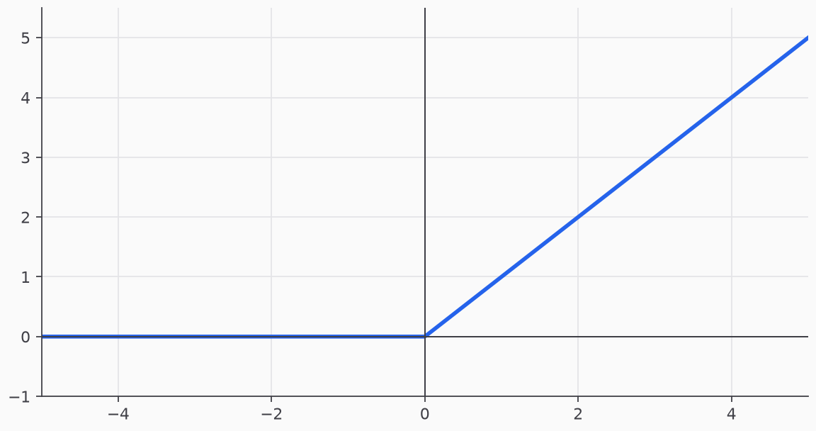
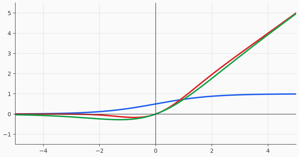
It is simple and cheap, but neurons that remain negative can stop receiving useful gradients. Near zero, a tiny change in the input can switch ReLU's gradient completely off or on. SiLU changes its gradient gradually instead, which can make optimization less sensitive to crossing this threshold.
Leaky ReLU
Leaky ReLU keeps a small slope for negative values:
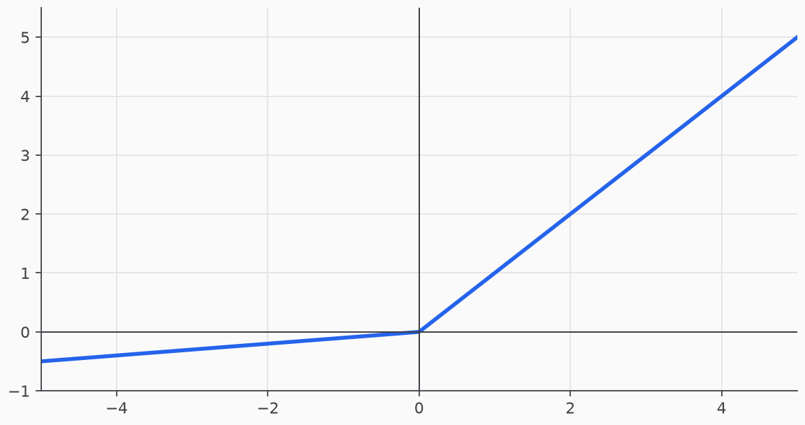
This reduces the risk of permanently inactive neurons while keeping ReLU's simplicity.
Sigmoid and tanh
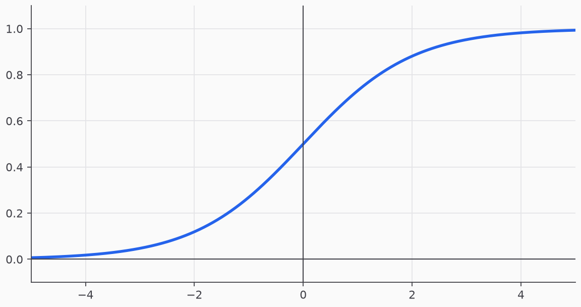
Sigmoid maps values to and is useful for gates and probabilities:
Tanh maps values to and is zero-centered:
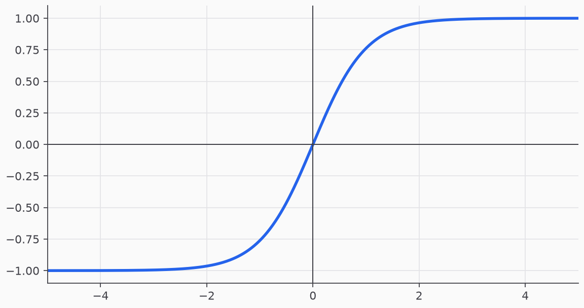
Both saturate for large positive or negative inputs, which can make their gradients very small.
GELU
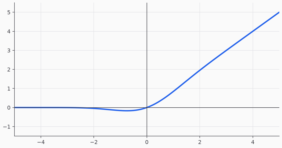
GELU smoothly gates values according to their magnitude instead of applying a hard cutoff. It is widely used in transformer models because its smooth behavior works well with gradient-based optimization.
where is the standard normal cumulative distribution function.
SiLU / Swish
SiLU, also called Swish, multiplies the input by its sigmoid:
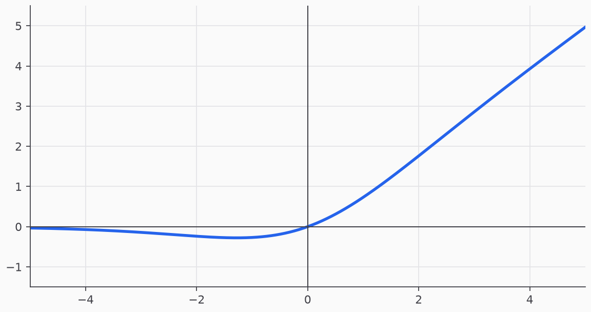
It is smooth and is commonly used in modern convolutional and language models.
GLU variants
Gated linear units split a projection into a value and a gate, then multiply them elementwise. For value projection and gate projection :
These are popular in transformers because the gate lets each token control how much of the value is passed through.
A standard dense Transformer MLP usually expands the hidden size to and projects it back, using roughly projection parameters. A GLU MLP has three projections: value, gate, and output. To keep its parameter count and matrix-multiplication cost close to the dense MLP, its intermediate width is commonly instead of . Although this width is smaller, the learned multiplicative gate gives the MLP more selective, conditional capacity, which is why SwiGLU often improves model quality at a similar compute budget.
For a dense MLP, the input and output projections have and parameters, respectively:
For a GLU with intermediate width , the value, gate, and output projections have , , and parameters:
Matching the dense MLP parameter count gives: